NAACL \(2022\) Interesting Papers & Workshop
In this short blog post, I will highlight a couple of interesting ideas presented in NAACL \(2022\).
♣ MCSE: Multimodal Contrastive Learning of Sentence Embedding
Humans rely on different modalities such as vision, language, and sound to capture an experience.
Recent works
Following previous trends, this work extends an existing sentence embedding method (i.e., SimSCE
The unsupervised SimSCE is used with dropout noise data augmentation. The model encodes the sentence twice using different dropout masks. For given sentence \(x_{i}\), the sentence is encoded twice via dropout masks \(\boldsymbol{h}_{i}^{z}=g_{\phi}\left(f_{\theta}\left(x_{i}, z\right)\right)\) and \(\boldsymbol{h}_{\dot{i}}^{z^{\prime}}=g_{\phi}\left(f_{\theta}\left(x_{i}, z^{\prime}\right)\right)\) where \(z\) and \(z^{\prime}\) refer to different dropout masks, \(f_{\theta}\) is a pre-trained language encoder BERT and \(g_{\phi}\) is the projection of the head after the [CLS] token. The training object can be written as:
\[ \small \ell_{i}^{S}=-\log \frac{e^{\operatorname{sim}\left(\mathbf{h}_{i}^{z_{i}}, \mathbf{h}_{i}^{z_{i}^{\prime}}\right) / \tau}}{\sum_{j=1}^{N} e^{\operatorname{sim}\left(\mathbf{h}_{i}^{z_{i}}, \mathbf{h}_{j}^{z_{j}^{\prime}}\right) / \tau}} \]where \(N \) is the mini-batch size, τ is the softmax temperature parameter and \(sim\) is the cosine similarity.
The next part is the integration of the visual feature. This work proposed a multimodal objective within the contrastive learning framework. For a given sentence-image \(x,y \) first they map \(x_{i} \) \( y_{i} \) into shared space:
\[ \small \boldsymbol{s}_{i}^{z}=g_{\phi_{1}}\left(f_{\theta}\left(x_{i}, z\right)\right), \boldsymbol{v}_{i}=g_{\phi_{2}}\left(f^{v}\left(y_{i}\right)\right) \] where \(f^{v}(\cdot) \) is a fixed pre-trained image encoder ResNet
The \( \lambda \) is the trade-off hyperparameter between the two objectives. The final loss with the two objectives:
\[ \small \ell_{i}=\ell_{i}^{S}+\lambda \ell_{i}^{M} \]Table 1 below shows the performance comparison on STS-B and SICK-R: SICK-Relatedness tasks. The results show the benefits of these visual representations in non-visual downstream tasks such as STS-B.
| Model | STSB | SICK-R |
| SimCSE-RoBERTa | 76.8 | 65.7 |
| MCSE-RoBERTa | 70.2 | 69.9 |
Also, the model is able to retrieve more descriptive captions as shown in Table 2 below.
| Model | Caption | |
| Query | A young girl is washing her teddy bear in the kitchen sink. | |
| SimCSE | A middle-aged woman is vacuuming her kitchen floor with a canister vac. | |
| MCSE | A young girl, blond and wearing a polka-dot shirt, washes a stuffed animal. |
♣ DiffCSE: Difference-based Contrastive Learning for Sentence Embeddings
Data augmentation with contrastive learning shows remarkable results in computer vision
This work uses equivariant contrastive learning from Computer Vision

In particular, they proposed an extension to SimSCE model with successful data augmentation with different prediction objectives that condition to the sentence embedding. For a given input sentence \(x\) the SimCSE provides a positive example via dropout masks and the same training objective:
\[\small \mathcal{L}_{\text {contrast }}=-\log \frac{e^{\operatorname{sim}\left(\mathbf{h}_{i}, \mathbf{h}_{i}^{+}\right) / \tau}}{\sum_{j=1}^{N} e^{\operatorname{sim}\left(\mathbf{h}_{i}, \mathbf{h}_{j}^{+}\right) / \tau}}, \] where \(N\) is the batch size for input batch, \(sim\) is the cosine similarity
function, and \(\tau\) is a hyperparameter. Then, As shown in Figure 1, to generate different conditional predictions an ELECTRA model
Then, after training, the model is optimized for the two losses (i.e., SimCSE and condition ELECTRA) with weight coefficient \(\lambda\).
\[ \small \mathcal{L}=\mathcal{L}_{\text {contrast }}+\lambda \cdot \mathcal{L}_{\text {RTD }} \]Table 1 below shows the benefits of using data augmentation techniques for sentence embedding tasks such as textual semantic similarity. This work also shows how data augmentation techniques can be applied for NLP tasks. Note that the original SimCSE demonstrates that different straightforward augmentation techniques (e.g., crop, word deletion, synonym replacement. etc.) can break the accuracy.
| Model | STS-B | SICK-R |
| SimCSE-RoBERTa | 77.24 | 71.16 |
| DiffCSE-RoBERTa | 82.38 | 71.19 |
♣ Fine-grained Image Captioning with CLIP Reward
Recent work uses CIDEr (i.e., text similarity) as a reward function to learn more descriptive image captions
where \(I\) and \(c\) refers to image and caption, \(f^{I}(I)\) and \(f^{T}(c)\) are the CLIP
image and text encoders. The captioning model \(P_{\theta}(c \mid I)\) is optimize using REINFORCE
where
\[ \small R(I, c)=\operatorname{CLIP}-\mathrm{S}(I, c) \]
However, this results in grammatically incorrect captions (e.g., word repetition) as CLIP is not trained on language model objective as shown in the example below in Table 1 on MS COCO karpathy test split.
| Reward | Caption | |
| CIDEr | a window of an airport with planes on the runway | |
| CLIP-S | several rows of planes packed outside a terminal window are with fog outside |
To address this, this work proposed to inject grammatical knowledge (grammar head) into CLIP encoder with randomly generated negative caption as noise (e.g., inserting/swapping/shuffling, etc.). In particular, a two-layer perceptron will take CLIP text feature \(f^{T}(c)\) as input and produces a probability \(c\) for grammatically correct caption with binary cross-entropy \(g(c) \in[0,1]\), where the grammar objective is labeled \(y = 1\) for reference captions and \(y = 0\) for the negative captions: \(−y\) log g(c):
\[ g(c)=\operatorname{sigmoid}\left(\operatorname{MLP}\left(f^{T}(c)\right)\right) \in[0,1] \]
Next, the model is jointly finetuned with the text encoder and grammar head using both the original CLIP and grammar head objectives. Finally, the captioning model is trained with the grammar score and the augmented reward:
\[ R(I, c)=\operatorname{CLIP}-\mathrm{S}(I, c)+\lambda g(c) \]
As shown in Table 2 below, the proposed CLIP-S+Grammar, the caption is more diverse than CIDEr as the model describes rainy weather with wet.
| Reward | Caption | |
| CIDEr | a window of an airport with planes on the runway | |
| CLIP-S | several rows of planes packed outside a terminal window are with fog outside | |
| CLIP-S+G | a lot of airplanes parked on a wet airport terminal |
♣ Progressive Class Semantic Matching for Semi-supervised Text Classification
This work shows the benefits of inherent semi-supervised knowledge into a pre-trained model
like BERT
ground truth class name: family
append word for this class: family
which is the best way to express ur love to ur girlfriend ? be a gentleman and
spending free time with her is ### 1 and be good listener
ground truth class name: Sport
append word for this class: Football
on may 27th 2006 did it have an NPA basketball game on tv ? yup miami 98 over detroit 83
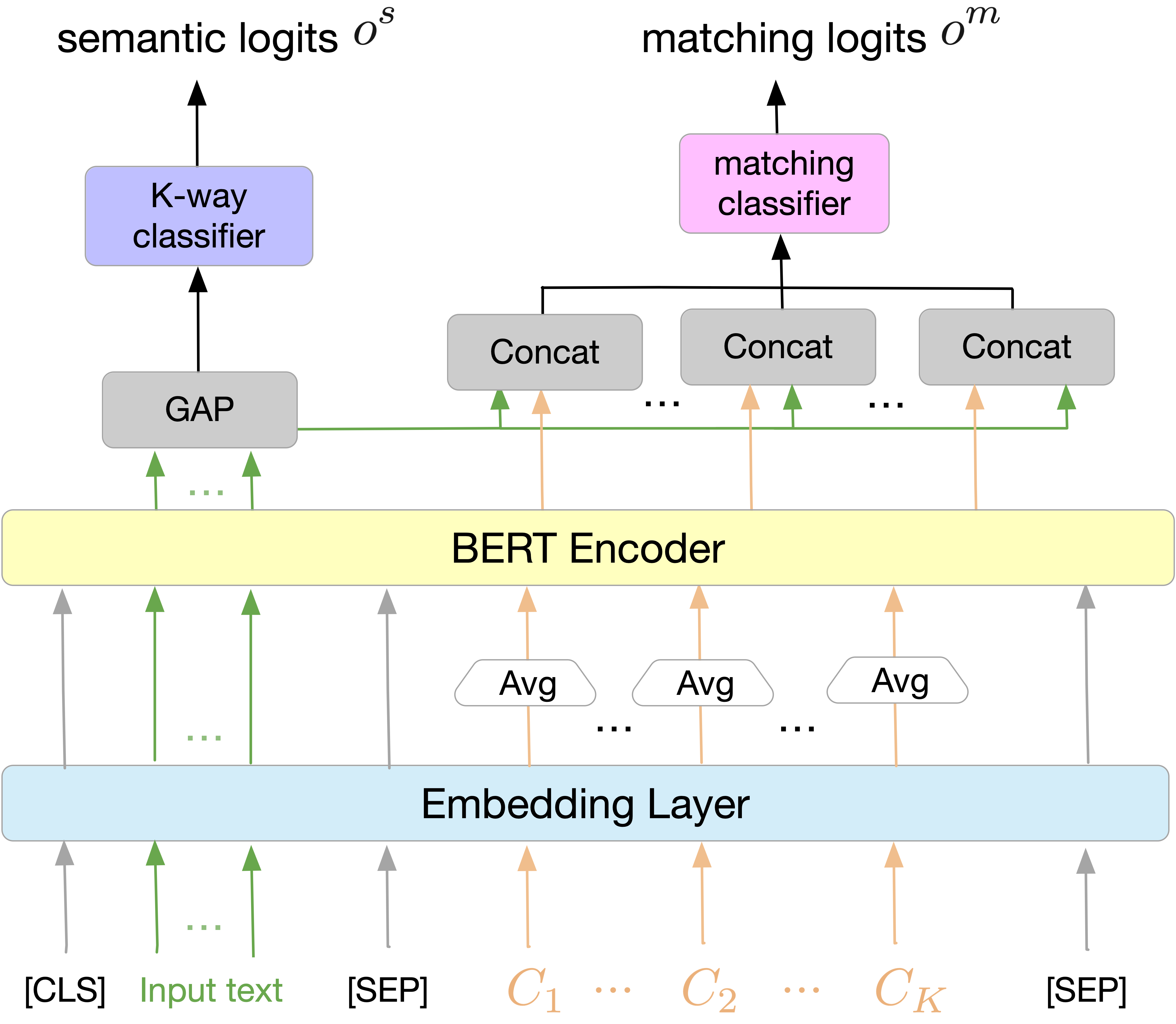
As shown in the figure below the proposed model Progressive Class-semantic Matching (PCM). The PCM is consist of three components: (1) class semantic representation \( C_{i} \), which constructs input to the BERT model by concatenating sentences with class semantic-related words; (2) standard K-way classifier with two-layer MLP with an output set as logits \(o_{i}^{s}\); (3) a class-sentence matching classifier via matching logits \( o_{i}^{m} \) via Sigmoid function to convert it into the probabilistic form.
The model relies on initialization stage of the classes-to-related words. Therefore, to initialize the class-related words \( C_{k} \) for PCM: (1) fine-tune K-way classifier on labeled data; pass labeled text into a fine-tuned model; (2) calculate attention value for each token; (3) retain top-\(j\) attend word for each class \( C_{k} \).

As shown in the example below the authors show some examples from AG news dataset. The proposed model can relate more accurate topics than fine-tuned topics BERT as shown in color red with unrelated topics.
word : world (from AG news)
init (BERT): bush, car, killed, black , story
Proposed: iraq, president , iraqi, military, troops
♣ Is Neural Topic Modelling Better than Clustering?
Recent Neural-based approaches
The proposed method can be summarized in the following steps: First, they (the authors) use pre-trained language models to obtain contextualized embeddings. Second, they apply K-Means to cluster similar documents (each cluster will be regarded as a topic). Third, they adopt a weighting method to select representative words as topics.
However, traditional TFIDF ignores the semantics between documents. To address this issue, two alternative strategies are considered: First, the authors concatenate the documents within a cluster to be a single long document and then calculate the term frequency of each word in each cluster:
\[ \small \mathbf{T}_{\mathbf{i}}=\frac{n_{t, i}}{\sum_{t^{\prime}} n_{t^{\prime}, i}} \]where \( n_{t,i}\) is the frequency of word \(t \) in cluster \(i\), \( \sum_{t^{\prime}} n_{t^{\prime}, i}\) is the total word frequency in the cluster \(i\). Second, for each cluster they apply:
\[ \small \mathbf{T F I D F}_{\mathbf{i}}=\frac{n_{t, d_{i}}}{\sum_{t^{\prime}} n_{t^{\prime}, d_{i}}} \cdot \log \left(\frac{\left|D_{i}\right|}{\left|\left\{d \in D_{i}: t \in d\right\}\right|}\right) \]where \( n_{t}, d_{i} \) refers to the frequency of word \( t \) in document \(d \) in cluster \(i\),\(|D_{i}|\)is number of documents in cluster \(i\).
Besides the two local cluster-based strategies, they further incorporate the global word importance with local term frequency within each cluster:
\[ \small \mathbf{ TFIDF } \times \mathbf{T F}_{\mathbf{i}}=\mathbf{T F I D F} \cdot \mathbf{T F}_{\mathrm{i}} \]And then combine the global word importance with term frequency across clusters:
\[ \small \mathbf{T F I D F} \times {\mathbf{I D F}_{\mathbf{i}}}=\mathbf{T F I D F}^{\operatorname{ID}} \log \left(\frac{|K|}{|\{t \in K\}|}\right) \]where \(|K|\) is the number of clusters and \(|\{t \in K\}|\) is the number of clusters that word \(t\) appears.
The proposed approach shows that directly clustering high-quality embeddings with an appropriate word selecting method can generate more coherent and diverse topics than recent neural topic models.
♣ Imagination-Augmented Natural Language Understanding
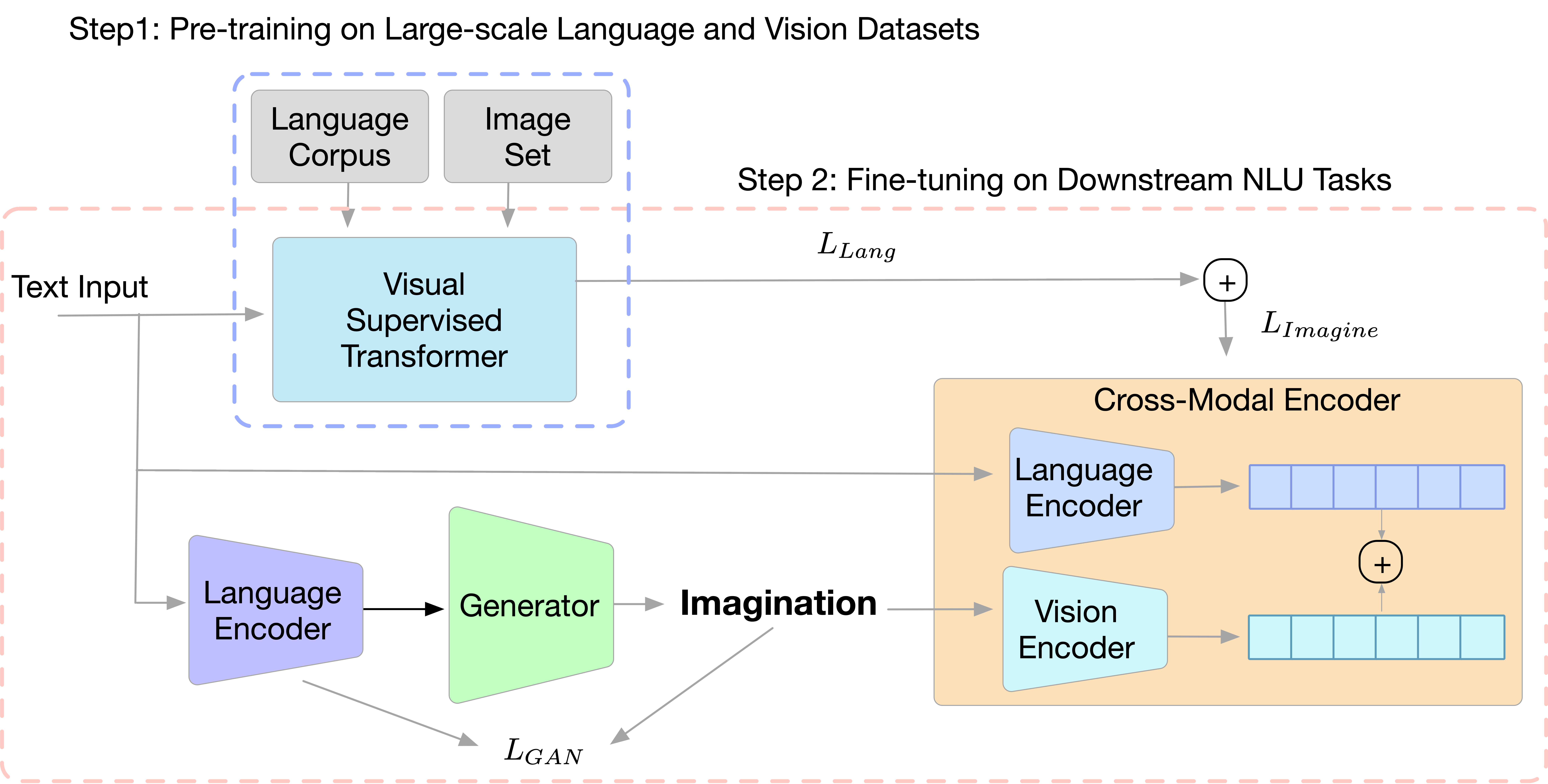
Humans understand language using visual imagination which fused two modalities in the brain to understand the language better. The neural activation, in the brain, of vision-related tasks is active when reading texts. This work tried to mimic human understanding via introducing a visual commonsense framework to pretrained multimodal models. The main idea is to use generated synthetic visual information using the text as an additional feature to the text itself to capture visual commonsense knowledge.
The model consists of three blocks as shown in Figure 1: (1) Image Generator: the GAN model is guided by CLIP model to generate relevant
images

Image Generator. Each piece of input text \(x\)
is treated as a prompt and VQGAN is used
The CLIP encodes the input text \(x\) and the corresponding imagination \(i\) as \(t\) and \(v\), and the training objective is to minimize the distance between \(t\) and \(v\) in the cross-modal embedding space.
Cross-Modal Encoder. The Cross-Modal Encoder takes the image and text and fuses them together.
The output will be representations of the imagination augmented in a bi-directional way. In particular, the Cross-Model
Encoder uses a vision transformer
where \(F\) denotes the set of regions of the imagination or the words of the textual sentence. \(W_{j}^{Q}\), \(W_{j}^{K}\) and \(W_{j}^{V}\), represents the weight in the \(j\)-th head for query, key, and value respectively. \(d_{k}\) is the dimension of the embedding. \(W\) is the weight matrix for multiple heads.
Then, they (the authors) apply late fusion on the text feature \(t\) and visual feature \(v\) to construct the cross-modal feature. Given the set of visual features \(S_{v}\) and textual features \(S_{t}\), the fused embedding \(X_{S}\) can be given:
\[\small X_{S}=\left[\operatorname{ReLU}\left(W_{t} S_{t}+b_{t}\right), \operatorname{ReLU}\left(W_{j} S_{v}+b_{j}\right)\right] \] Visually-Supervised Transformer. VOKEN
Learning Procedure. The learning procedure is divided into two steps: (1) pre-trained the visually supervised Transformer, and (2) fine-tune the proposed framework with imagination on downstream tasks.
Step 1: Visually-Supervised Transformer. As we mentioned above, VOKEN proposed a voken classification task. Given a set of tokens with masks, the model is asked to predict the best-matching image (the voken) for each token. The pre-training loss can be given as: \[\small {L}=-\lambda_{1} \sum_{w_{j} \in \hat{s}} \log q_{j}\left(w_{j} \mid \check{s}\right)-\lambda_{2} \sum_{w_{j} \in \hat{s}} \log p_{j}\left(v\left(w_{j} ; s\right) \mid \check{s}\right) \]
here \(s\) is the token set, \(\check{s}\) is the mask tokens. and \(\hat{s}\) is the unmasked tokens. The \(q_{j}\) and \(p_{j}\) refer to the conditional probability of the \(j\)-th token given token \(w_{j}\) and voken \(v(w_{j} ; s) \) respectively. The \(\lambda\)s are the balance factor of the Mask Language Model and voken-classification task. The Voken enables the matching between the general language token and its related image from COCO dataset.
Step 2: Imagination-augmented Fine-tuning: The fine-tuning is performed on downstream tasks like GLUE with cross-entropy loss:
\[\small {L}_{\text {Imagine }}=-\sum_{j=1}^{|D|} \sum_{k=1}^{K} y_{k} \log p_{k}\left(d_{j}(\boldsymbol{t} ; \boldsymbol{v}) \mid D\right) \]where \(j\) refer to the \(j\)-th data sample in the dataset \(D\), \(K\) is the class number, \(p_{k}\) represents the conditional probability of \(d_{j}\). The model relies only on the language model during the fine-tuning:
\[\small {L}_{\text {Lang }}=-\sum_{j=1}^{|D|} \sum_{k=1}^{K} y_{k} \log p_{k}\left(d_{j}(\boldsymbol{t}) \mid D\right) \]Finally, the imagination-augmented loss and language model loss is summed up with balanced factor \( \lambda \)s during the training:
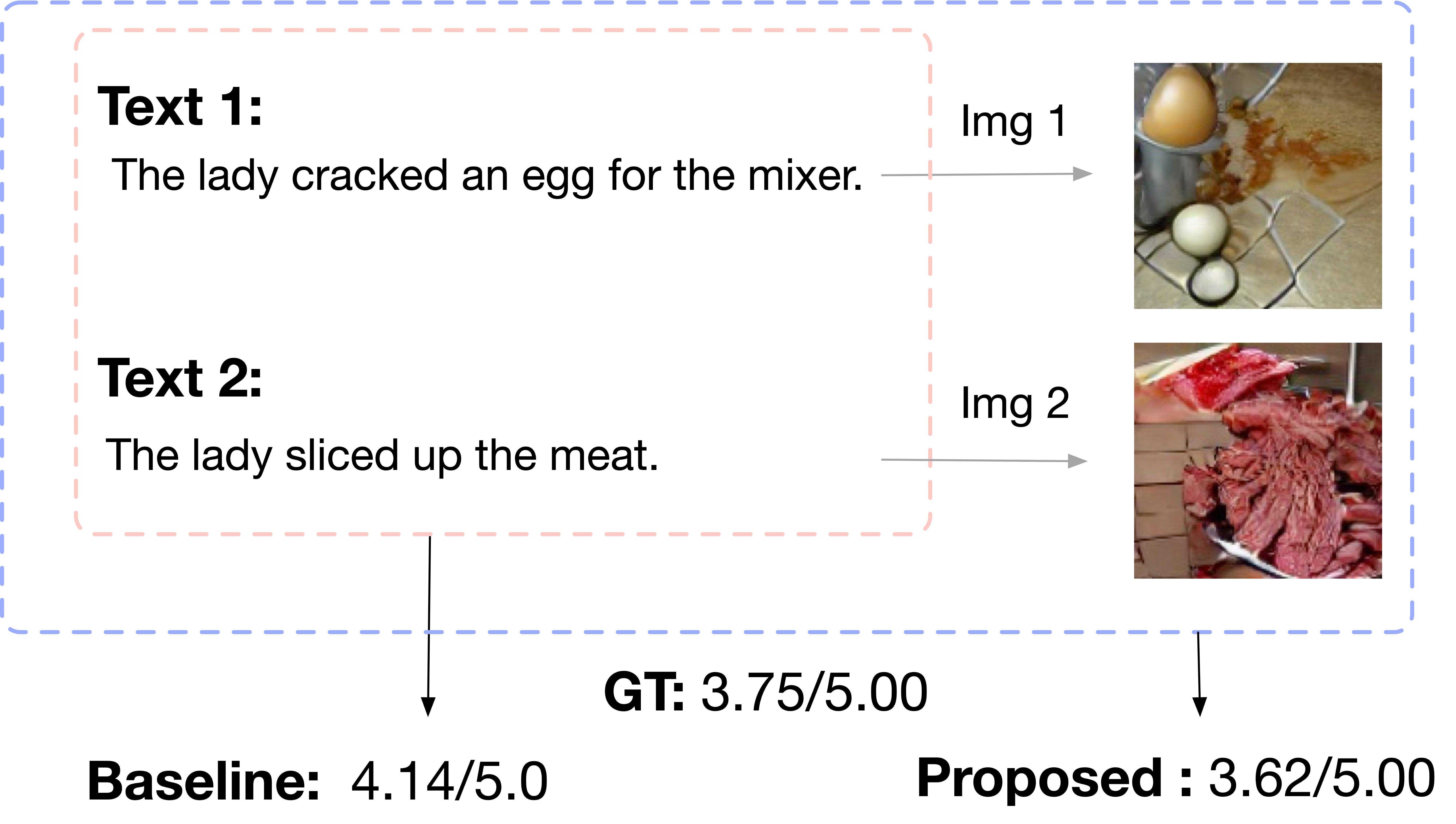
\[ {L}=\lambda {L}_{\text {Imagine }}+(1-\lambda){L}_{\text {Lang }} \]Figure 2 below shows that adding visual information imagination-augmented helps give the model a context and thus the predictions are more aligned with human score.

♣ SURF: Semantic-level Unsupervised Reward Function for Machine Translation
Machine Translation suffers from objective mismatch during the training and the inference.
During the training, the teacher forces the generation to be conditioned on the target sequence
using cross-entropy with Maximum Likelihood Estimation objective (MLE). However, during the inference,
the generation is conditioned on the previous outputs. In addition, unlike during the training,
the model loss is evaluated using MLE Loss, but at inference time the model is evaluated using
standard metrics like BLEU
This work applied Reinforcement Learning agents (RL) to bridge the gap between training and inference. In particular, the agent as a state takes the previous sequence \(\hat{y}_{1:t-1} \) and takes an action on the current token \(\hat{y}_{t} \), then after generating the token the agent gives a reward from the environment which is commonly defined (e.g., BLEU). Thus, the objective of this work is to maximize the expected reward by the evaluation metric like BLEU.
One of the problems of using an RL for this task is the capability of generalization of the agent to explore hypotheses in the hypothesis space. This work proposed an unsupervised reward function with normalized measures that assessed both sentences in fluency and semantic diversity and ensure the reward is uniform and can be generalized to out-of-the-domain data. The two rewards functions are the incremental difference between the two pay-off functions (reward shaping) are:
Sentence Fluency (F). The F reward is defined as the average Log-Likelihood of the generated sequence. Each term is the probability of a token given the previous one (generated tokens). The score is computed using a pre-trained Language Model.
\[\small \frac{1}{\tau} \log \prod_{t}^{\tau} p\left(\hat{y}_{t} \mid \hat{y}_{1: t-1}\right) \]where \(\hat{y}_{1:t}\) is the generated sequence at timestep \(t\). The F function determines the effectiveness of the generated token a time step in respect of the current/previous sentence as a reward function.
Sentence-level Semantic Similarity (SLSS).
The SLSS is the cosine similarity between Cross-lingual Embedding between the source and the target language (generated sequence)
Finally, to ensure the uniformity across all source sequences the score is normalized with respect to the target sequence.
Workshop
→ Using Natural Sentence Prompts for Understanding Biases in Language Models
Most previous work, uses simple template to mimic the real sentences (e.g., The {man/woman} laughed because .. ) for gender bias evaluation. However, these template is too simple and can trigger gender-specific continuations. This work proposed a real synthetic dataset for gender bias evaluation using prompts. This dataset is used to study biases between profession definitions and gender in language models as shown below.
A silversmith is a metalworker
who crafts objects from silver
<- Original sentence
A person is a metalworker
who crafts objects from silver
where .. <- Final prompt
A dermatologist is a specialist doctor
who manages diseases related to skin, hair and nails and some cosmetic problems.
<- Original sentence
A dermatologist is a person
who manages diseases related to skin, hair and nails
where .. <- Final prompt
The findings of this paper are: (1) the gender bias evaluations are sensitive to the template prompts, and (2) the default behavior of language models is already biased.
→ How do people talk about images? A study on open-domain conversations with images
This work analyzed conversations with images in open domain scenario (ImageChate dataset)
| Related | Utterance | Image |
|---|---|---|
| Yes | Never had this food before and not sure if I’m ready to try it today. | 
|
| No | That’s it, I going to Vegas tomorrow. Who’s coming with me?s | 
|
This study shows that the noise that comes from images-caption extracted from the web without a strict filter. Most recent model such as CLIP is trained on this kinda data, and thus these pairs (no relation between image and the associated text) introduce noise to the model.